Subsections

• FM Modulation
• FM Demodulation

Introduction

FM Modulation

In angle modulation, the amplitude of the signal is held constant and the phase is being varied with the message. An angle modulated signal is of the form:

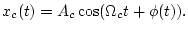$$x_c(t)=A_c\cos(\Omega_c t+\phi(t)).$$ (1)

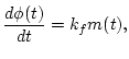
The instantaneous phase of $x_c(t)$ is given by

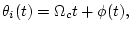$$\theta_i(t)=\Omega_c t+\phi(t),$$ (2)

and the instantaneous frequency is given by

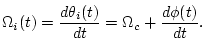$$\Omega_i(t)=\frac{d\theta_i(t)}{dt}=\Omega_c+\frac{d\phi(t)}{dt}.$$ (3)

Using this approach, if the message is proportional to $\phi(t)$, which is the phase deviation, then we have phase modulation. If the message is proportional to $\frac{d\phi(t)}{dt}$, which is the frequency deviation, then we have frequency modulation.

In order to have phase modulation,

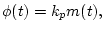$$\phi(t)=k_p m(t),$$ (4)

where $k_p$ is known as the deviation constant. For frequency modulation,

$$\frac{d\phi(t)}{dt}=k_f m(t),$$ (5)

where $k_f$ is known as the frequency deviation constant. Consequently, an FM modulated signal is of the form

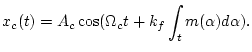$$x_c(t)=A_c\cos(\Omega_c t + k_f\int_t m(\alpha)d\alpha).$$ (6)

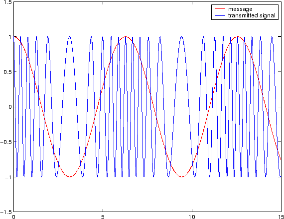
An FM signal is shown in Figure 1

Figure 1: Frequency modulation

FM Demodulation

There are several ways to demodulate an FM signal. In this lab you will use a differentiator followed by an AM detector do demodulate and FM signal as shown in Figure 2

Figure 2: Frequency discriminator

In order to implement the above the frequency discriminator, we need to design a differentiator. One way to implement a differentiator is using an optimal equiripple linear-phase FIR filter. This filter is optimal because the weighted approximation error between the desired frequency response and the actual frequency response is spread evenly across the passband and evenly across the stopband. This results in minimizing the maximum error. Remez algorithm may be used to generate this filter. Below are samples of the output generated using the firpm function.

Figure 3: Magnitude repines FIR equiripple differentiator for $\omega =0$ to $0.4\pi$

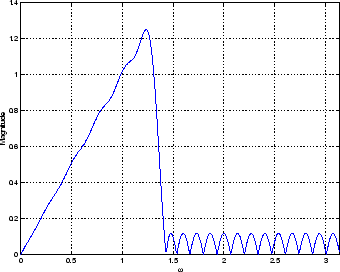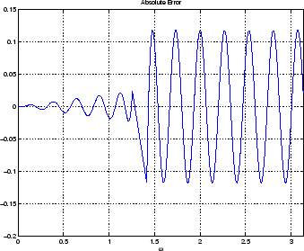
Figure 4: Absolute error of an FIR equiripple differentiator for $\omega =0$ to $0.4\pi$